VE-IFR transformation

In many cases, we don’t have the full set of information needed to create the fully correct, reality reflecting tables for everything. The final fueling decision is a series of multiplications and divisions, thus allowing for ‘the fudge factor’—we can account for imprecisions by artificially altering other values. MAP and TEMP are fed from sensors, so short of upgrading the sensors themselves, we don’t have a way to influence their precision. AFR is just an arbitrary divider that we can verify with a wideband oxygen sensor. As long as that sensor is properly calibrated, there’s nothing to fudge there either. VE or GMVE, paired up with IFR are very frequently used to make up for imprecisions. VE is not easily measured, and IFR as my recent fuel pressure investigations indicate, is more complicated that we originally thought. IFR however can be calculated, if we have enough data for it. So if we have all variables except VE and IFR, and we can calculate IFR, we should be able to arrive at a reasonably realistic VE. Since VE is such a crucial table, it’s worth the extra effort to arrive at the higher precision version of it.

Let’s start with understanding of what a good tune is: a collection of final fueling decisions that result in desired target AFR. No matter how much fudging in tables is involved, it’s possible to arrive at it the final figures in an infinite number of combinations—that’s what most ‘professionals’ tune, they do not concern themselves with the truthfulness of numbers, just with the final resulting AFR. While effective, I’d like to enhance our ability to arrive at the precise numbers that reflect reality.

Fuel decisions are nothing else but a set of Injector Pulse Widths calculated for every possible condition encountered in our engine. We calculate them using the formula:

IPW = GMVE*MAP/(AFR*IFR*TEMP)

So to convert from one set of parameters that creates a good tune, to another set of parameters that yield the same IPW’s, this must be true:

IPWnew = IPWold

So we expand both sides of this equality:

GMVEnew * MAPnew /(AFRnew * IFRnew * TEMPnew) = GMVEold * MAPold / (AFRold * IFRold * TEMPold)

And then solve it for the new GMVE:

GMVEnew = GMVEold * (MAPold/MAPnew) * (AFRnew/AFRold) * (IFRnew/IFRold) * (TEMPnew/TEMPold)

We notice that if the tune is good, if it preserves the final fueling, target AFRs will be the same, thus:

(AFRnew/AFRold) = 1

Temperatures are also the same across the full range, TEMPnew/TEMPold = 1

Same goes for MAP ranges, MAPold/MAPnew = 1

This simplifies the main equation to:

GMVEnew =GMVEold * (IFRnew/IFRold)

Also notice that since

GMVE = Vol * VE / R

and Vol and R are constants, thus:

VEnew =VEold * (IFRnew/IFRold)

This means this transformation applies to both VE and GMVE forms, allowing the same logic and methodology to be applied to LS1/LS6 and the newer LS2 computers.

The important thing to remember here is that while these equations work for singular values, these dependencies must be true across the full table.

IFRold-3D version

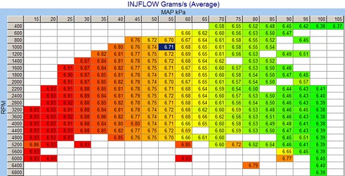
The easiest way to visualize that is by employing the histograms. We’re all used to looking at the VE table and IFR tables, that’s nothing new. Here, in order to multiply them all out just like the formulas would suggest, all the variables in question must be describing the same temporal instance in the engine. Then in order to perform the calculation, we also must have it in the same units. IFRold is the traditional IFR table, but viewed not in a traditional 2D way, referenced against Manifold Vacuum, but on the same axis as the VE table. How do we view it this way? The easiest way is to log GM.INJFLOW, and then make a custom histogram, starting with your basic BEN histogram, but then changing the data to be working on GM.INJFLOW, not BENs. This will give you a VE-like view of what injector flow the computer uses to calculate the final fueling. Displaying of the actual histogram is optional, it’s not mandatory for the final transformation to work, but it does help to understand what we’re doing here, and why do we need to grow a whole new dimension on a simple IFR table.



IFRnew

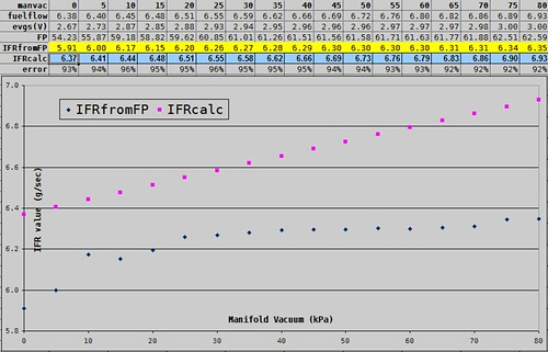
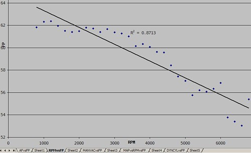
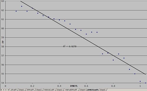
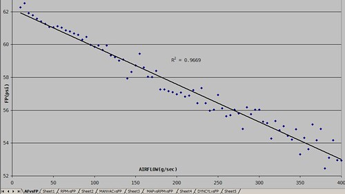
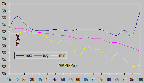
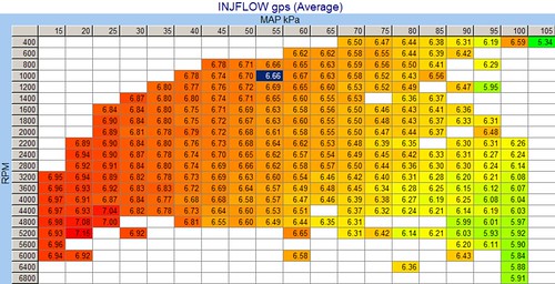
The tricky part is how we arrive at the IFRnew. As I found out from the Under (Fuel) Pressure write-up, Fuel Pressure varies not only based on Manifold Vacuum, but also on RPM and even smaller factors, like the Battery Voltage. Thus, to obtain the most realistic IFR table, we also must create a histogram that takes these variables into consideration, and then shape it just like the IFRold histogram we created in previous paragraph, to be able to do an element-wise division, for the final calculation. Just like IFRold histogram, this one is also optional, and one purely for educational purposes.

First we must log the Fuel Pressure. Hardware and setup necessary to do that is beyond the scope of this write-up, as it’s been wonderfully described in TAquickness’ document . Once we have CALC.FUEL_PRESSURE (or whatever other name you gave it, I’m going to use this name in this document for clarity), we need to create another custom PID that calculates the injector flow based on the injector rating, Manifold Vacuum, and the Fuel Pressure.

EFILive’s custom PID infrastructure allows us to do all this, and even have multiple units for the same entity.

First we add few units to calc_pids.txt:

*UNITS

#Code System Abbr Description

#-------- ---------- -------- -------------------------------------------------------------

PSI Imperial PSI "Pounds Per Square Inch"

KPA Metric KPA "kilo Pascals"

GPS Metric gps "grams per second"

LBPM Imperial lbpm "pounds per minute"

unit Metric unit "unit"

Then we create calculated PIDs for converting FP gauge voltage to PSI and KPA. This example uses GM.EGRS as the source of FP voltage, as per example in TAquickness write-up. If you have it hooked up through the external inputs, please refer to his manual how to adjust this PID definition.

*CLC-00-001

PSI 0.00 100 .2 "({GM.EGRS}*25)-12.5"

KPA 0.0 700 .1 "(({GM.EGRS}*25)-12.5)*6.89475728"

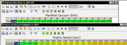
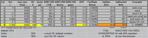
Now we must calculate our own CALC.INJFLOW which is calculated from GM.MANVAC and CALC.FUEL_PRESSURE. Notice that in order for the calculations to make sense, they all are converted to kPa.

*CLC-00-002

GPS 0.0000 30 .4 "42*0.125997778*sqrt(({GM.MANVAC.kPa}+{CALC.FUEL_PRESSURE.KPA})/(3*100))"

LBPM 0.000 200 .3 "42* sqrt(({GM.MANVAC.kPa}+{CALC.FUEL_PRESSURE.KPA})/(3*100))"

Notice that this is the place where we must hardcode the value for the rated flow and pressure of the injectors.

The 42 at the beginning is an example of a popular 42 lb/hr injector. This is where you insert the rating of the injector in lb/hr, and the conversion to g/sec is done for you. The rated fuel pressure is at the end, that’s the (3*100). Most injectors I’ve seen are rated at 3bar, and to convert from bar to kPa you just multiply by 100. So unless you have some really unusual injectors, you most likely will not need to change this, this is just for your information.

There are two versions of the same PID, this way we can display the calculated injector flow in both popular units for easier understanding.

Now set up another histogram, again with the usual VE axis (I like to use the BEN histogram as a starting point), and replace BEN’s with the CALC.INJFLOW.



Marcin Transformation Factor

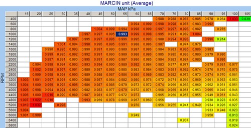
We have now two histograms of IFR—one is the IFRold, and the second is IFRnew. We can create another calculated PID that will divide the two tables on element-by-element basis.

*CLC-00-003

unit 0.000 10 .3 "{CALC.INJFLOW.GPS}/{GM.INJFLOW.gps}"

And finish it off with the PRN section that binds all the previous definitions into coherent entities:

# ==============================================================================

*PRN - Parameter Reference Numbers

# --------------------------------

# See sae_generic.txt for more information on the *PRN section

#

#Code PRN SLOT Units System Description

#------------------------- ---- ------------ ---------------- ---------------- ------------------------------------------

CALC.FUEL_PRESSURE F001 CLC-00-001 "PSI,KPA" Fuel "Fuel Pressure"

CALC.INJFLOW F002 CLC-00-002 "GPS,LBPM" Fuel "Injector Flow from Fuel Pressure"

CALC.MARCIN F003 CLC-00-003 unit Fuel "Marcin Transform"

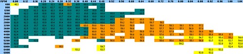
With the complete setup, we should create the final histogram—yes you guessed it again, on the same VE-like axis. This time, we use CALC.MARCIN for the data to histogram. You should get a histogram that has a bunch of values near 1.0. The more your Fuel Pressure was varying from the theoretical based pressure we used to use with the old IFR spreadsheet, the farther away from 1.0 the corrections are going to be. This histogram is mandatory.



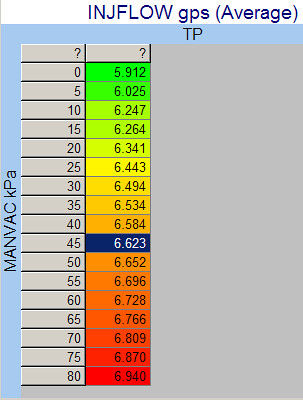
IFRnew-2D

The other important thing that you can get from all these calculated PIDs, is the automatic creation of your new, Fuel Pressure based IFR. All you need to do is create another histogram, with CALC.INJFLOW as data, and GM.MANVAC as rows with 0..80kPa range with 5kPa step. This histogram is also mandatory. This is what you’re going to paste into {B4001} table.

Now you can copy the whole CALC.MARCIN table, and multiply it out with your existing VE {B0101} table, transforming it to account and agree with the IFR table that we just build in the paragraph above. Together, the new VE and IFR should preserve the final fueling, which if you had it perfect to start with, should carry over to the new setup.




Conclusions

While not instantly mind blowing, these concepts and tools have some deep consequences. Now you are able to convert any VE into another VE based on a different, hopefully better, IFR settings. This means, if you have a tune done by some hack tuner that jacked up your VE and IFR arbitrarily, you can log Fuel Pressure, and painlessly and without full VE tuning sessions, transform into a much cleaner, saner and meaningful, closer to reality VE and IFR tables.

Another application is playing with Fuel Pressure, or installing a new Fuel Pressure Regulator, on your already well tuned configuration. Normally, you’d have to start from scratch, and tuning VE yet another time. This allows you to be able to play with the FPR much more, looking for the perfect base and rising rate to compromise between good low pulse width idle quality, and regulating FP so at WOT you have a safe amount of fuel provided to the injectors. You can just try yet another IFR setup and see what it will do to your VE with no need for slow, ticket-prone retunes.

If you suspect your fuel system isn’t up to task, logging fuel pressure and histogramming it as described in this write-up will also show you the deficiencies. At this point you can either chose to just use the transformation described and account for the deficiencies, or go shopping for a more capable system. The important part here is, you don’t have to guess and eyeball anymore, you can quantify it and see it in black and white.

Side notes and Commentary

All of this is done in EFILive, no spreadsheets, no custom code, just utilizing a well designed infrastructure. This little exercise demonstrates just how powerful it can be. About 12hrs before I had the first functional Transformation Matrix, I never set up a custom PID. So it cannot be that difficult either.

On the other hand, we have HPTuners. I got some data with logged fuel pressure voltage, and while I was able to convert the voltage into actual Fuel Pressure, converting from BARO and MAP into MANVAC turned out to be outside of its reach. I’ve spent hours experimenting with it, trying to get it to work, with no results. I tried to refer to some other more hardcore HPTuners users out there, and not only they weren’t able to set it up, It also turned out to be really difficult to exchange the custom PIDs, as there is no clear configuration file containing such info. If anyone knows how to deal with these issues with HPTuners, please let me know, I’d love to have another version of document that explains it in HPTuners terms.

I highly recommend learning to harness the power of custom PIDs and custom histograms; this is how the raw data turn into information.

Special thanks goes out to a prof of mine, Mathias Kolsch, who in the process of teaching me Computer Vision, gave me lots of new tools and ideas, some of which directly contributed to this particular transformation method.

Big thanks also go out to TAquickness and Tordne, who had the insight to set up fuel pressure logging, and patience to explain all the EFILive intricacies to me, as well as being crazy enough to let me test my theories on their cars.

On a more personal note, this is probably going to be the last writeup for another 6 months, as I must finish my masters degree and write a thesis. I'd rather be tuning, but oh well. This isn't a complete retirement, I am trying to take some classes in which I could spend improving my tools (Human Computer Interaction), and learn more math to spot and analyze relationships in data (Data Analysis and Simulation) so there will be updates, just nothing huge.

Keep warm, and happy New Years,
Marcin

Fuel Pump sizing

My fuel pump pressure post gave me a lot to think about, and few people had some interesting questions as well. One of the simplest, yet most important questions was 'is the fuel pump holding up?' I looked around, and amazingly, I have not found much information on how to estimate how much fuel your fuel pump needs to be able to pump so injectors can keep with the demand.

Most fuel pumps are rated in how many Liters of fluid they can pump an hour. I'm not exactly sure why they'd go with a volume flow rating, when injectors are mass flow rated. The easy way around it is to convert one to the other, which should be easy, as mass=density*volume. Of course there are various types of gas, so the density specific to particular types of petrol will differ, but the generally we should be close to desired rating. I found numbers of 690g/L to 770g/L, so I'm going to use 730 for an easy average. These translate to 0.690kg/m^3, 0.770kg/m^3 and 0.730kg/m^3 respectively, for the more traditional measure of densities.

This spreadsheet converts the rated flow of the pump into units comparable with the units used for injectors, and then divides the flow of the pump by the number of injectors, to see if the flow provided to each injector is larger than what the injector would flow at WOT at standard LSx 58psi fuel pressure.

It's all very simple, but the funny part is that once I started plugging in typical fuel pump flows, the per injector flows were very closely matched to the flows provided by the popular injector sizes!


190 lb/hr fuel pump outputs just above what SVO red tops need.
255 lb/hr fuel pump outputs just above what SVO green tops need.
350lb/hr fuel pump outputs just above what Mototron 60's need.

I'm not sure if it's coincidence or not, but it works so nicely, it's a really easy 'rule of thumb' to match injectors with pumps for a well balanced system.

Here's the DOWNLOAD if you want to play with more specific options.

More fuel system investigations coming soon.
Stay tuned,
Marcin

IFR spreadsheet for Logged Fuel Pressure

Here's the new, promised IFR spreadsheet that calculates IFR table accounting for the variable Fuel Pressure.

DOWNLOAD

This is NOT a replacement for the old IFR spreadsheet! This is only for people who set up their Fuel Pressure sender units to log. If you don't have such a setup, continue using the old one.

Remember that this will only work if you log your fuel pressure first against a variety of driving conditions. I'm not going to describe how to log it, as I've already seen it set up as the EGR voltage, or as the separate input (just like a wideband). HPTuners and EFILive setups differ as well, so deal with it appropriately. I don't have resources to describe every possible combination of hardware and software here, and this is a more advanced thing to do anyway, so I'd rather not give people a false sense of assurance.

One important note: remember that most pressures in the GM PCM are absolute. IFR for some strange reason, is based not on MAP just like about anything else, but on Manifold Vacuum. In EFILive this is easy, MANVAC is just another PID to pick. In HPTuners, I haven't seen it yet. I tried to make it with a custom PID of BARO-MAP, and then use it to create a custom histogram of the new MANVAC-like PID against the Fuel Pressure PID. Easier said than done, after many hours and help from people that know HPT in and out, I just gave up. This is what you get for hacking custom PIDs into HPT at the last moment, and not having them as a part of design and infrastructure from the get go.
Anyway... If anyone figures out how to get FP vs MANVAC histogram going in HPT without major hacks, please let me know, right now it's a bloody mess.

Just like I mentioned in the last writeup, FP apparently varies even within the same MAP range, making tuning IFR against the logged Fuel Pressure closer to The Truth(TM) but still not perfect. For now, we're still stuck dealing with the VE table making up for non-MAP related IFR variations.

Next up: transforming VE's using the new IFR without retuning.
Stay tuned,
Marcin

Under (Fuel) Pressure

After a year and a half of using the IFR spreadsheet, I came to the conclusion that while it is not wrong as far as the information given, it leaves much to be desired when it comes to truly reflecting reality. The biggest problem it has is the lack of expressing how fuel pressure differs at various loads (Manifold Vacuum).

Unexplainably high VE values on some cars made me think that even though we 'fixed' some old-school arbitrary IFR choices, we're still fudging somewhere, because there's no reason for the theoretical VE numbers to be that high.
Once I created the equations for airflow I realized that the only spot where the 'fudge factor' could occur would be the IFR. The rest of terms in the eqations is either logged (MAP, temps, RPM) or not exactly changable (number of cylinders, cylinder displacement). In the meantime, TAQuickness and few others started working on a simple setup that would allow us to log fuel pressure alongside all the usual PIDs, not just a simple gauge you can look at at idle.
Eventually all the experiments came together, and provided me with some very interesting data. The car from which the logs discussed here come from is running 42lb/hr@3bar injectors running at 63psi. On the table and chart below, the values calculated using the standard IFR spreadsheet are labled IFRcalc (pink dots, values on blue background). The other data series is calculated from logged Fuel Pressure (comes in as a EGR voltage, so it's evgs in the table) which then gets converted to PSI for easy lookup/calculations (marked FP).
Once we know the nominal flow of the injectors and the real Fuel Pressure, we can calculate the real flow of injectors (labeled IFRfromFP, blue dots, yellow background in the table)
As you can see, the blue dots are nowhere near pink dots. Apparently measuring the fuel pressure at idle (no load) doesn't give you the best numbers. That's fine, that means you just need to reconfigure IFR for new FP, right? Wrong!
Not only the FP numbers going in aren't close to what they are, they are also non-linear. We need to update the IFR spreadsheet to be able to take various FP inputs, depending on the MAP. Easy enough I think, and quickly make some adjustments to the spreadsheets.



The Fuel Pressure drop seemed significant enough that I wanted to understand it deeper, it didn't just seem to be some underpowered aftermarket junk part, but a more complex issue. I wasn't quite convinced that the Fuel Pressure drop was solely a function of MAP/Manifold Vacuum. So I started graphing FP against various entities to get a better feel for it.
There was an obvious relationship between MAP/Manifold Vacuum and FP, as we already have seen with the data above.
I graph it against RPM, and there's another definite relationship. Now I'm confused--how can it be, if the crucial IFR table is purely manifold pressure based?



Another popular view is airmass based, like the timing tables, I thought, maybe it's load/compression/torque dependent, afterall that's when the most air gets consumed.



I graph FP vs DynCylAir and I keep getting the same shape drop when I did when I graphed it against RPM. Why not do a 3D graph of FP vs RPM and DynCylAir? I'm starting to see a cleaner relationship, the more DynCylAir coupled with RPM the less FP we get.




So I'm thinking: DynCylAir is like torque, and DynAir is like horsepower, and TQ and HP are bound through RPM, so why not graph DynAir vs FP?



BINGO! This graph seems to be very linear, with a high degree of confidence.
But then I start to think what does this mean--why higher Airflow makes the Fuel Pressure drop so consistently linear? Obvieously more airflow needs more fuel flow, they're coupled through the AFR, RPM just enforces the time intervals to do the fuel injection in, and IFR tailors it to the injector size and fuel pressure.
From the Speed Density paper I've discovered that:

AIRFLOW=CYL*RPM*IPW*AFR*IFR/120
and we know that
IFR=IFR(rated)*sqrt(FP/FP(rated))

which for the purpose of this discussion(meaning keeping everything else constant) means that Airflow is directly proportional to RPM, and the square root of Fuel Pressure. This is not what this graph says, at least with the given precision. This graph, even though introduces a lot more noise for the high Airflow values, still seems to lay along a straight line. So the possible explanation might be that because we're using a fairly small range of FP values, we don't get see the curve that would result from a square root relationship.
Another explanation comes from the way I obtained the data for the Airflow vs FP graph itself; I histogrammed the Airflow into 5g/sec bins, to equalize the number of samples along the axis, because it's hard to log large number of samples in higher airflow ranges on the street. If I fit a line to a large number of samples, mostly in the lower ranges, the fit would be good there, but the scarse upper range data would be largely ignored. While the histogramming first gets rid of the weighing to the large number of samples problems, it potentially loses a lot of precision, in our case enough to not be able to tell which type of relationship it is.

So this investigation leaves us with more questions than answers:

1. Why does the FP drops so much more than it officially supposed to (proportional only to MAP)
2. If the FP is so well proportioned to Airflow, is that by design or by accident?
3. Even if I log FP precisely for my fuel system and adjust IFR values directly based on that, the swings if FP values within the same MAP range (since that's all we can differenciate by in the IFR table), are still significant.
   
   
   
   The only table that's able to account for the RPM swings is VE. This is not what I wanted to achive here, I wanted to free the VE table to be the 'catch all fudge table' and have it become the true theoretical Volumetric Efficiency. So where else could I move the fudging duty to?

The good part is that now we know just how bad our fuel systems are when trying to hold up to a moderate (400lb/min of airflow ain't that much, I've seen cam-only LS2's flowing 450+) power. Throw in a better flowing system, more cubes, or god forbid any forced induction, and our FP shrinks down in the moments when we need it most--WOT. So, if you want to impulse buy anything this xmas, I highly recommend a return fuel system with a manifold pressure referenced fuel pressure regulator.


This investigation started really small, I just wanted to see how badly does the Fuel Pressure drop and what effect it has on the IFR. Now I see the shortcomings of the fuel systems, computer's inability to express all the changes that take place, and shortcomings of my own IFR spreadsheet (new version coming up shortly).
There will definitely be a lot of other stuff coming out of these observations, as this is very scary, considering how much trust we put in aftermarket pumps, and they simply fall short of expectations. I've always told people to get bigger injectors and run with a healthy margin left. Apparently I didn't know just how right I was--in this case running with IFR falling 10psi from what your computer knows about yields 9% less fuel delivered! When you're trying to get your AFR within 1-2%, 9% error in one of your data is going to seriously monkey wrench your system.

So this xmas, be afraid, be very afraid...

New IFR spreadsheet, and then automatic translation of your VE based on the new IFR are going to be the next targets of attack for me toolwise.

Stay tuned,
Marcin

Why tune VE?

This is a post in one of the forums, I usually don't like to duplicate information, but singular forums posts tend to get lost in the noise, so I'm posting it up here as this is something that should be very clear to everyone that's trying to tune their car.

The question was:
Does this (VE tuning) gain me anything performance wise?


This is a very good question, I'm glad someone is trying to understand what it is that VE tuning is actually about, not just how to do it.

1. Without VE being perfect, you'll never be able to find out proper timing. When computer detects the tiniest tendency to run lean, it will be very trigger happy to pull timing with usually no good reason. Thus, if your VE is on the lean side (and it usually is, after all that's what adding better flowing parts is about--flowing more air) you will get a lot of knock in random spots, and no amount of pulling timing yourself will cure it, causing your car run like poo.
2. Sudden transitions are hard to get right. Without VE being dead on, you are making it almost impossible to get right. Bad transitions cause knock, which lingers around, doesn't last just when going over the areas that aren't perfectly tuned. I've seen knock last over 5 secs. If you're a drag racer, that's diminished performance for half of your run. That's why it's also important to tune not just some of the VE, but ALL of it.
3. When your car develops a problem, you will notice it. If your VE is well done. airflow numbers will be down, knock will appear, but you know it's not the fault of the bad tune, but a result of some hardware component failing.
4. When VE is perfect, it is meaningful. If you add a part that supposed to improve engine's breathing, your VE will go up, and if you get it tuned perfectly before and after, you will know just how well the part works, and for what MAP/RPM range.
5. With perfect VE, your airmass and airflow numbers will be meaningful as well. with their close correspondence to torque and horsepower respectively, you can optimize your powerband.
6. Perfect VE enforces other tables to be meaningful as well. For example, to obtain the same proper fueling with wrong VE, you will have to hack either your IFR or PE numbers. With all of them perfect and meaningful, when you want a 12.9AFR, you can just command it in PE and it will happen, instead of taking stabs in the dark hoping that some arbitrary PE will make it happen by accident.
7. Since VE dictates airmass and airflow, everything based off such tables will work better as well. Shift tables for automatics need to know how much power you're really making. If you're lying about VE, then this power estimation is also wrong, making the transmission misbehave.

In general, VE in itself is important. A lot of other things are derived by calculations based on numbers calculated from VE. It really ends up being a domino effect. If VE is meaningful and proper, then it forces other things to meaningful and proper as well. But if you botch/ignore VE, then the bad effects will propagate, making the entire tune a major hack, making the car drive horribly, and sending the tuner chasing his tail. You pick which domino effect you'd rather experience.

In the long run it's really just easier to do it Right.

Unscrewing a bad tune, Part 2

Sunday mornings are usually connected to fuzzy slippers, eggs and bacon, extra long lounging session in the tub...but not today. Barely did I sit down in front of my computer, I was asked to look at some Forced Induction tunes. The guy asking these questions was rather skeptical about the correctness of some examples he's received. Of course, the people who he got the tunes were claiming their turbo setups running well.

So I dove into one of the tunes, and all the usual marks of a bad tune were there: arbitrary IFR, untouched VE and MAF curves, super aggressive PE triggers. The whole tune was pretty much based on the PE table, assuming identical boost and airflow at the same RPM, and ignoring all other variables. The car supposedly was running well at 10psi, making me wonder if I can learn something from it. In order to do that, I decided to 'unscrew' the hacked up tune. If the measured AFR was correct, that would indicate that the final fueling decisions were made correctly, despite the wrong input data. Since this is a staple of every 'pro' tuner out there, I decided to see if it's possible to see if two wrongs can make a right.

Since the car was running in MAF mode, and the MAF signal completely maxed out by applying some healthy 10psi, I knew that the airflow figures are going to be wrong. While looking at the IFR table, I learned that the injector flow values were completely arbitrary. PE was the only real tuning device, and the resulting Pulse Width was the only non-wrong, non-fake value in the whole setup. Thus, task 1: calculate the IPW.



This part is easy, I thought. Plug in the wrong numbers, in my case 59lb/min of airflow (max'ed out MAF), 41.3lb/hr injectors, 11.15 PE value for 6400rpm which was the redline, into my VE2IPW calculator and be done. I realized that's no so easy, as my VE2IPW calculator is optimized for working with Speed Density data, not MAF. There is no field for Airflow, only its components, and Airflow gets calculated dynamically behind the scenes. I looked into the Speed Density paper for some equations, but they were no help either, as they also expected either VE, GMVE, or rho (air density), and I didn't have any of them available. If you want the hairy math details, read the updated paper. If you don't, here's a short version:

IPW=120*Airflow/(Cyl*RPM*AFR*IFR)

This means now we can calculate Pulse Width directly from the airflow number, no matter what the source of it might be, MAF or Dynamic Airflow are both fully viable sources. In the case of the hacked up FI tune I knew the car ran on maxed out MAF, so I just used the maximum value from the MAF table, 59.8 lb/hr. Few quick unit conversions and simple math operations later, I arrive at the IPW at 6400RPM: 18.9 msec.



OK, so now what? I figured I wanted to first see what the numbers would really look like if the tune was done properly. I inversed the formula to calculate the Airflow from IPW:

Airflow= IPW*Cyl*RPM*AFR*IFR/120

The big change this time I wasn't going to go with fake, ridiculous PE and arbitrary IFR. I found out what the injectors really were, calculated their flow against the fuel pressure I was told the car ran at (48.5 lb/hr). I used the AFR values from what the car supposedly ran at, 12.0AFR. Again, do some unit conversions, and out pops out the real value for airflow we should get: 576g/sec (75.6 lb/min), which is beyond the max value storable in the MAF table. So yet again, MAF being useless on Forced Induction comes out again.

Then I decided to compare this estimation of the real airflow with one of my older spreadsheets (INJsize.xls) to see how close the two are.

So I quickly punched in 8 cylinders, 5.3L (it was a truck tune), 6400rpm redline, 100%VE, and 10psi of boost. The result says 576.7 g/sec (76.1 lb/min) of airflow. That's within 1% I was happy to see consistency between the two completely different methods arriving at the same conclusion. Of course, a quick glance at the injector sizing spreadsheet pointed out that he needs almost 100% of fuel flow capacity of 48.5 lb/min injectors, and that to make it go down to 80%, he'd need to flow about 60 lb/min. Another popular myth busted--you can't run much of a FI setup on the popular 42 lb/hr (@3bar) injectors, need to step up to something bigger.



I'm posting the updated Speed Density paper HERE, and the example 'bad2good' spreadsheet HERE.

happy unscrewing bad tunes,
Marcin